Part 1: Boosting and Ensembling
We are now going to look at ways in which multiple machine learning can be combined.
In particular, we will look at a way of combining models called boosting.
Review: Components of A Supervised Machine Learning Problem
At a high level, a supervised machine learning problem has the following structure:
$$ \underbrace{\text{Training Dataset}}_\text{Attributes + Features} + \underbrace{\text{Learning Algorithm}}_\text{Model Class + Objective + Optimizer } \to \text{Predictive Model} $$
Review: Overfitting
Overfitting is one of the most common failure modes of machine learning.
- A very expressive model (a high degree polynomial) fits the training dataset perfectly.
- The model also makes wildly incorrect prediction outside this dataset, and doesn't generalize.
Review: Bagging
The idea of bagging is to reduce overfitting by averaging many models trained on random subsets of the data.
for i in range(n_models):
    # collect data samples and fit models
    X_i, y_i = sample_with_replacement(X, y, n_samples)
    model = Model().fit(X_i, y_i)
    ensemble.append(model)

# output average prediction at test time:
y_test = ensemble.average_prediction(y_test)
The data samples are taken with replacement and known as bootstrap samples.
Review: Underfitting
Underfitting is another common problem in machine learning.
- The model is too simple to fit the data well (e.g., approximating a high degree polynomial with linear regression).
- As a result, the model is not accurate on training data and is not accurate on new data.
Boosting
The idea of boosting is to reduce underfitting by combining models that correct each others' errors.
- As in bagging, we combine many models $g_t$ into one ensemble $f$.
- Unlike bagging, the $g_t$ are small and tend to underfit.
- Each $g_t$ fits the points where the previous models made errors.
Weak Learners
A key ingredient of a boosting algorithm is a weak learner.
- Intuitively, this is a model that is slightly better than random.
- Examples of weak learners include: small linear models, small decision trees.
Structure of a Boosting Algorithm
The idea of boosting is to reduce underfitting by combining models that correct each others' errors.
- Fit a weak learner $g_0$ on dataset $\mathcal{D} = \{(x^{(i)}, y^{(i)})\}$. Let $f=g_0$.
- Compute weights $w^{(i)}$ for each $i$ based on model predictions $f(x^{(i)})$ and targets $y^{(i)}$. Give more weight to points with errors.
- Fit another weak learner $g_1$ on $\mathcal{D} = \{(x^{(i)}, y^{(i)})\}$ with weights $w^{(i)}$.
- Set $f_1 = g_0 + \alpha_1 g$ for some weight $\alpha_1$. Go to Step 2 and repeat.
In Python-like pseudocode this looks as follows:
weights, ensemble = np.ones(n_data,), Ensemble([])
for i in range(n_models):
    model = SimpleBaseModel().fit(X, y, weights)
    predictions = ensemble.predict(X)
    model_weight, weights = update_weights(weights, predictions)
    ensemble.add(model, model_weight)

# output consensus prediction at test time:
y_test = ensemble.predict(y_test)
Origins of Boosting
Boosting algorithms were initially developed in the 90s within theoretical machine learning.
- Originally, boosting addressed a theoretical question of whether weak learners with >50% accuracy can be combined to form a strong learner.
- Eventually, this research led to a practical algorithm called Adaboost.
Today, there exist many algorithms that are considered types of boosting, even though they're not derived from the perspective of theoretical ML.
Algorithm: Adaboost
- Type: Supervised learning (classification).
- Model family: Ensembles of weak learners (often decision trees).
- Objective function: Exponential loss.
- Optimizer: Forward stagewise additive model building.
Defining Adaboost
One of the first practical boosting algorithms was Adaboost.
We start with uniform $w^{(i)} = 1/n$ and $f = 0$. Then for $t=1,2,...,T$:
- Fit weak learner $g_t$ on $\mathcal{D}$ with weights $w^{(i)}$.
- Compute misclassification error $e_t = \frac{\sum_{i=1}^n w^{(i)} \mathbb{I}\{y^{(i)} \neq f(x^{(i)})\}}{\sum_{i=1}^n w^{(i)}}$
- Compute model weight $\alpha_t = \log[(1-e_t)/e_t]$. Set $f \gets f + \alpha_t g_t$.
- Compute new data weights $w^{(i)} \gets w^{(i)}\exp[\alpha_t \mathbb{I}\{y^{(i)} \neq f(x^{(i)})\} ]$.
Adaboost: An Example
Let's implement Adaboost on a simple dataset to see what it can do.
Let's start by creating a classification dataset.
# https://scikit-learn.org/stable/auto_examples/ensemble/plot_adaboost_twoclass.html
import numpy as np
from sklearn.datasets import make_gaussian_quantiles

# Construct dataset
X1, y1 = make_gaussian_quantiles(cov=2., n_samples=200, n_features=2, n_classes=2, random_state=1)
X2, y2 = make_gaussian_quantiles(mean=(3, 3), cov=1.5, n_samples=300, n_features=2, n_classes=2, random_state=1)
X = np.concatenate((X1, X2))
y = np.concatenate((y1, - y2 + 1))
We can visualize this dataset using matplotlib.
import matplotlib.pyplot as plt
plt.rcParams['figure.figsize'] = [12, 4]

# Plot the training points
plot_colors, plot_step, class_names = "br", 0.02, "AB"
x_min, x_max = X[:, 0].min() - 1, X[:, 0].max() + 1
y_min, y_max = X[:, 1].min() - 1, X[:, 1].max() + 1

for i, n, c in zip(range(2), class_names, plot_colors):
    idx = np.where(y == i)
    plt.scatter(X[idx, 0], X[idx, 1], cmap=plt.cm.Paired, s=60, edgecolor='k', label="Class %s" % n)
plt.xlim(x_min, x_max)
plt.ylim(y_min, y_max)
plt.legend(loc='upper right')
<matplotlib.legend.Legend at 0x12afda198>

Let's now train Adaboost on this dataset.
from sklearn.ensemble import AdaBoostClassifier
from sklearn.tree import DecisionTreeClassifier

# Create and fit an AdaBoosted decision tree
bdt = AdaBoostClassifier(DecisionTreeClassifier(max_depth=1),
                         algorithm="SAMME",
                         n_estimators=200)
bdt.fit(X, y)
AdaBoostClassifier(algorithm='SAMME',
                   base_estimator=DecisionTreeClassifier(max_depth=1),
                   n_estimators=200)
Visualizing the output of the algorithm, we see that it can learn a highly non-linear decision boundary to separate the two classes.
xx, yy = np.meshgrid(np.arange(x_min, x_max, plot_step), np.arange(y_min, y_max, plot_step))

# plot decision boundary
Z = bdt.predict(np.c_[xx.ravel(), yy.ravel()])
Z = Z.reshape(xx.shape)
cs = plt.contourf(xx, yy, Z, cmap=plt.cm.Paired)

# plot training points
for i, n, c in zip(range(2), class_names, plot_colors):
    idx = np.where(y == i)
    plt.scatter(X[idx, 0], X[idx, 1], cmap=plt.cm.Paired, s=60, edgecolor='k', label="Class %s" % n)
plt.xlim(x_min, x_max)
plt.ylim(y_min, y_max)
plt.legend(loc='upper right')
<matplotlib.legend.Legend at 0x12b3b8438>

Ensembling
Boosting and bagging are special cases of ensembling.
The idea of ensembling is to combine many models into one. Bagging and Boosting are ensembling techniques to reduce over- and under-fitting.
- In stacking, we train $m$ independent models $g_j(x)$ (possibly from different model classes) and then train another model $f(x)$ to prodict $y$ from the outputs of the $g_j$.
- The Bayesian approach can also be seen as form of ensembling $$ P(y\mid x) = \int_\theta P(y\mid x,\theta) P(\theta \mid \mathcal{D}) d\theta $$ where we average models $P(y\mid x,\theta)$ using weights $P(\theta \mid \mathcal{D})$.
Pros and Cons of Ensembling
Ensembling is a useful tecnique in machine learning.
- It often helps squeeze out additional performance out of ML algorithms.
- Many algorithms (like Adaboost) are forms of ensembling.
Disadvantages include:
- It can be computationally expensive to train and use ensembles.
Pros and Cons of Boosting
Boosting algorithms generalize Adaboost and offer many advantages:
- High accuracy via a highly expressive non-linear model family.
- Low pre-processing requirements if trees are used as weak learners.
Disadvantages include:
- Large ensembles can be expensive to train.
- The interpretability of the weak learners is lost.

Part 2: Additive Models
Next, we are going to see another perspective on boosting and derive new boosting algorithms.
The Components of A Supervised Machine Learning Algorithm
We can define the high-level structure of a supervised learning algorithm as consisting of three components:
- A model class: the set of possible models we consider.
- An objective function, which defines how good a model is.
- An optimizer, which finds the best predictive model in the model class according to the objective function
Review: Underfitting
Underfitting is another common problem in machine learning.
- The model is too simple to fit the data well (e.g., approximating a high degree polynomial with linear regression).
- As a result, the model is not accurate on training data and is not accurate on new data.
Review: Boosting
The idea of boosting is to reduce underfitting by combining models that correct each others' errors.
- As in bagging, we combine many models $g_i$ into one ensemble $f$.
- Unlike bagging, the $g_i$ are small and tend to underfit.
- Each $g_i$ fits the points where the previous models made errors.
Additive Models
Boosting can be seen as a way of fitting an additive model: $$ f(x) = \sum_{t=1}^T \alpha_t g(x; \phi_t). $$
- The main model $f(x)$ consists of $T$ smaller models $g$ with weights $\alpha_t$ and paramaters $\phi_t$.
- The parameters are the $\alpha_t$ plus the parameters $\phi_t$ of each $g$.
This is more general than a linear model, because $g$ can be non-linear in $\phi_t$ (therefore so is $f$).
Example: Boosting Algorithms
Boosting is one way of training additive models.
- Fit a weak learner $g_0$ on dataset $\mathcal{D} = \{(x^{(i)}, y^{(i)})\}$. Let $f=g_0$.
- Compute weights $w^{(i)}$ for each $i$ based on model predictions $f(x^{(i)})$ and targets $y^{(i)}$. Give more weight to points with errors.
- Fit another weak learner $g_1$ on $\mathcal{D} = \{(x^{(i)}, y^{(i)})\}$ with weights $w^{(i)}$.
- Set $f_1 = g_0 + \alpha_1 g$ for some weight $\alpha_1$. Go to Step 2 and repeat.
Forward Stagewise Additive Modeling
A general way to fit additive models is the forward stagewise approach.
- Suppose we have a loss $L : \mathcal{Y} \times \mathcal{Y} \to [0, \infty)$.
- Start with $f_0 = \arg \min_\phi \sum_{i=1}^n L(y^{(i)}, g(x^{(i)}; \phi))$.
- At each iteration $t$ we fit the best addition to the current model. $$ \alpha_t, \phi_t = \arg\min_{\alpha, \phi} \sum_{i=1}^n L(y^{(i)}, f_{t-1}(x^{(i)}) + \alpha g(x^{(i)}; \phi))$$
Practical Considerations
- Popular choices of $g$ include cubic splines, decision trees and kernelized models.
- We may use a fixed number of iterations $T$ or early stopping when the error on a hold-out set no longer improves.
- An important design choice is the loss $L$.
Exponential Loss
Give a binary classification problem with labels $\mathcal{Y} = \{-1, +1\}$, the exponential loss is defined as
$$ L(y, f) = \exp(-y \cdot f). $$
- When $y=1$, $L$ is small when $f \to \infty$.
- When $y=-1$, $L$ is small when $f \to - \infty$.
Let's visualize the exponential loss and compare it to other losses.
from matplotlib import pyplot as plt
import numpy as np
plt.rcParams['figure.figsize'] = [12, 4]

# define the losses for a target of y=1
losses = {
    'Hinge' : lambda f: np.maximum(1 - f, 0),
    'L2': lambda f: (1-f)**2,
    'L1': lambda f: np.abs(f-1),
    'Exponential': lambda f: np.exp(-f)
}

# plot them
f = np.linspace(0, 2)
fig, axes = plt.subplots(2,2)
for ax, (name, loss) in zip(axes.flatten(), losses.items()):
    ax.plot(f, loss(f))
    ax.set_title('%s Loss' % name)
    ax.set_xlabel('Prediction f')
    ax.set_ylabel('L(y=1,f)')
plt.tight_layout()

Special Case: Adaboost
Adaboost is an instance of forward stagewise additive modeling with the expoential loss.
At each step $t$ we minimize $$L_t = \sum_{i=1}^n e^{-y^{(i)}(f_{t-1}(x^{(i)}) + \alpha g(x^{(i)}; \phi))} = \sum_{i=1}^n w^{(i)} \exp\left(-y^{(i)}\alpha g(x^{(i)}; \phi)\right) $$ with $w^{(i)} = \exp(-y^{(i)}f_{t-1}(x^{(i)}))$.
We can derive the Adaboost update rules from this equation.
Suppose that $g(y; \phi) \in \{-1,1\}$. With a bit of algebraic manipulations, we get that: \begin{align*} L_t & = e^{\alpha} \sum_{y^{(i)} \neq g(x^{(i)})} w^{(i)} + e^{-\alpha} \sum_{y^{(i)} = g(x^{(i)})} w^{(i)} \\ & = (e^{\alpha} - e^{-\alpha}) \sum_{i=1}^n w^{(i)} \mathbb{I}\{{y^{(i)} \neq g(x^{(i)})}\} + e^{-\alpha} \sum_{i=1}^n w^{(i)}.\\ \end{align*} where $\mathbb{I}\{\cdot\}$ is the indicator function.
From there, we get that: \begin{align*} \phi_t & = \arg\min_{\phi} \sum_{i=1}^n w^{(i)} \mathbb{I}\{{y^{(i)} \neq g(x^{(i)}; \phi)}\} \\ \alpha_t & = \log[(1-e_t)/e_t] \end{align*} where $e_t = \frac{\sum_{i=1}^n w^{(i)} \mathbb{I}\{y^{(i)} \neq f(x^{(i)})\}}{\sum_{i=1}^n w^{(i)}\}}$.
These are update rules for Adaboost, and it's not hard to show that the update rule for $w^{(i)}$ is the same as well.
Squared Loss
Another popular choice of loss is the squared loss. $$ L(y, f) = (y-f)^2. $$
The resulting algorithm is often called L2Boost. At step $t$ we minimize $$\sum_{i=1}^n (r^{(i)}_t - g(x^{(i)}; \phi))^2, $$ where $r^{(i)}_t = y^{(i)} - f(x^{(i)})_{t-1}$ is the residual from the model at time $t-1$.
Logistic Loss
Another common loss is the log-loss. When $\mathcal{Y}=\{-1,1\}$ it is defined as:
$$L(y, f) = \log(1+\exp(-2\cdot y\cdot f)).$$
This looks like the log of the exponential loss; it is less sensitive to outliers since it doesn't penalize large errors as much.
from matplotlib import pyplot as plt
import numpy as np
plt.rcParams['figure.figsize'] = [12, 4]

# define the losses for a target of y=1
losses = {
    'Hinge' : lambda f: np.maximum(1 - f, 0),
    'L2': lambda f: (1-f)**2,
    'Logistic': lambda f: np.log(1+np.exp(-2*f)),
    'Exponential': lambda f: np.exp(-f)
}

# plot them
f = np.linspace(0, 2)
fig, axes = plt.subplots(2,2)
for ax, (name, loss) in zip(axes.flatten(), losses.items()):
    ax.plot(f, loss(f))
    ax.set_title('%s Loss' % name)
    ax.set_xlabel('Prediction f')
    ax.set_ylabel('L(y=1,f)')
    ax.set_ylim([0,1])
plt.tight_layout()

In the context of boosting, we minimize $$J(\alpha, \phi) = \sum_{i=1}^n \log\left(1+\exp\left(-2y^{(i)}(f_{t-1}(x^{(i)}) + \alpha g(x^{(i)}; \phi)\right)\right).$$
This gives a different weight update compared to Adabost. This algorithm is called LogitBoost.
Pros and Cons of Additive Models
The algorithms we have seen so far improve over Adaboost.
- They optimize a wide range of objectives.
- Thus, they are more robust to outliers and extend beyond classification.
Cons:
- Computational time is still an issue.
- Optimizing greedily over each $\phi_t$ can take time.
- Each loss requires specialized derivations.
Summary
- Additive models have the form $$ f(x) = \sum_{t=1}^T \alpha_t g(x; \phi_t). $$
- These models can be fit using the forward stagewise additive approach.
- This reproduces Adaboost and can be used to derive new boosting-type algorithms.
Part 3: Gradient Boosting
We are now going to see another way of deriving boosting algorithms that is inspired by gradient descent.
Review: Boosting
The idea of boosting is to reduce underfitting by combining models that correct each others' errors.
- As in bagging, we combine many models $g_i$ into one ensemble $f$.
- Unlike bagging, the $g_i$ are small and tend to underfit.
- Each $g_i$ fits the points where the previous models made errors.
Review: Additive Models
Boosting can be seen as a way of fitting an additive model: $$ f(x) = \sum_{t=1}^T \alpha_t g(x; \phi_t). $$
- The main model $f(x)$ consists of $T$ smaller models $g$ with weights $\alpha_t$ and paramaters $\phi_t$.
- The parameters are the $\alpha_t$ plus the parameters $\phi_t$ of each $g$.
This is not a linear model, because $g$ can be non-linear in $\phi_t$ (therefore so is $f$).
Review: Forward Stagewise Additive Modeling
A general way to fit additive models is the forward stagewise approach.
- Suppose we have a loss $L : \mathcal{Y} \times \mathcal{Y} \to [0, \infty)$.
- Start with $f_0 = \arg \min_\phi \sum_{i=1}^n L(y^{(i)}, g(x^{(i)}; \phi))$.
- At each iteration $t$ we fit the best addition to the current model. $$ \alpha_t, \phi_t = \arg\min_{\alpha, \phi} \sum_{i=1}^n L(y^{(i)}, f_{t-1}(x^{(i)}) + \alpha g(x^{(i)}; \phi))$$
Limitations of Forward Stagewise Additive Modeling
Forward stagewise additive modeling is not without limitations.
- There may exist other losses for which it is complex to derive boosting-type weight update rules.
- At each step, we may need to solve a costly optimization problem over $\phi_t$.
- Optimizing each $\phi_t$ greedily may cause us to overfit.
What Do Weak Learners Learn?
Consider, for example, L2Boost, which optimizes the L2 loss $$ L(y, f) = \frac{1}{2}(y-f)^2. $$
At step $t$ we minimize $$\sum_{i=1}^n (r^{(i)}_t - g(x^{(i)}; \phi))^2, $$ where $r^{(i)}_t = y^{(i)} - f_{t-1}(x^{(i)})$ is the residual from the model at time $t-1$.
Recall that the residual is $$r^{(i)}_t = y^{(i)} - f_{t-1}(x^{(i)})$$
Observe that the residual is also the derivative of the $L2$ loss $$\frac{1}{2}(y^{(i)} - f_{t-1}(x^{(i)}))^2$$ with respect to $f$ at $f_{t-1}(x^{(i)})$: $$r^{(i)}_t = \frac{\partial L(y^{(i)}, \text{f})}{\partial \text{f}} \bigg\rvert_{\text{f} = f_{t-1}(x)}$$
Thus, at step $t$ we minimize $$\sum_{i=1}^n \left( \underbrace{\left(y^{(i)} - f_{t-1}(x^{(i)})\right)}_\text{derivative of $L$ at $f_{t-1}(x^{(i)})$} - g(x^{(i)}; \phi)\right)^2. $$
Why does L2Boost fit the derivatives of the L2 loss?
A High-Level Look at Supervised Learning
To explain this phenomenon, let's first recap classical supervised learning, and then contrast it against a different approach (gradient boosting).
Supervised Learning: The Model
Recall that a machine learning model is a function $$ f_\theta : \mathcal{X} \to \mathcal{Y} $$ that maps inputs $x \in \mathcal{X}$ to targets $y \in \mathcal{Y}$.
The model has a $d$-dimensional set of parameters $\theta$: $$\theta = (\theta_1, \theta_2, ..., \theta_d). $$
Supervised Learning: The Learning Objective
Intuitively, $f_\theta$ should perform well in expectation on new data $x, y$ sampled from the data distribution $\mathbb{P}$:
$$ J (\theta) = \mathbb{E}_{(x, y)\sim \mathbb{P}} \left[ L\left( y, f_\theta( x \right)) \right] \text{ is "good"}. $$
Here, $L : \mathcal{X}\times\mathcal{Y} \to \mathbb{R}$ is a performance metric and we take its expectation or average over all the possible samples $ x, y$ from $\mathbb{P}$.
Recall that formally, an expectation $\mathbb{E}_{x\sim {P}} f(x)$ is $\sum_{x \in \mathcal{X}} f(x) P(x)$ if $x$ is discrete and $\int_{x \in \mathcal{X}} f(x) P(x) dx$ if $x$ is continuous.
Intuitively, $$J(\theta) = \mathbb{E}_{(x, y)\sim \mathbb{P}} \left[ L\left( y, f_\theta( x) \right) \right] = \sum_{x \in \mathcal{X}} \sum_{y \in \mathcal{Y}} L\left(y, f_\theta(x) \right) \mathbb{P}(x, y) $$ is the performance on an infinite-sized holdout set, where we have sampled every possible point.
Supervised Learning: The Optimizer (Gradient Descent)
The gradient $\nabla J(\theta)$ is the $d$-dimensional vector of partial derivatives:
$$ \nabla J (\theta) = \begin{bmatrix} \frac{\partial J(\theta)}{\partial \theta_1} \\ \frac{\partial J(\theta)}{\partial \theta_2} \\ \vdots \\ \frac{\partial J(\theta)}{\partial \theta_d} \end{bmatrix}.$$
The $j$-th entry of the vector $\nabla J (\theta)$ is the partial derivative $\frac{\partial J(\theta)}{\partial \theta_j}$ of $J$ with respect to the $j$-th component of $\theta$.
We can optimize $J(\theta)$ using gradient descent via the usual update rule: $$\theta_t \gets \theta_{t-1} - \alpha_t \nabla J(\theta_{t-1}).$$
However, in practice, we cannot measure $$\nabla J(\theta) = \mathbb{E}_{( x, y)\sim \mathbb{P}} \left[ \nabla L\left( y, f_\theta( x) \right) \right]$$ on infinite data.
We substitute $\nabla J(\theta)$ with an approximation $\hat \nabla J(\theta)$ measured on a dataset $\mathcal{D}$ sampled from $\mathbb{P}$: $$ \hat \nabla J (\theta) = \frac{1}{m} \sum_{i=1}^m \nabla L\left( y^{(i)}, f_\theta( x^{(i)}) \right). $$ If the number of IID samples $m$ is large, this approximation holds (we call this a Monte Carlo approximation).
A High-Level Look at Supervised Learning Over Functions
Instead of finite-dimensional paramters, we can try optimizing directly over infinite-dimensionals functions $$ f : \mathcal{X} \to \mathcal{Y} $$ from inputs $x \in \mathcal{X}$ to targets $y \in \mathcal{Y}$.
This will give us the gradient boosting algorithm.
Supervised Learning Over Functions: The Model
Our model space is now the (unrestricted) set of functions $f: \mathcal{X} \to \mathcal{Y}$:
Each function is an infinite-dimensional vector indexed by $x \in \mathcal{X}$: $$ f = \begin{bmatrix} \vdots \\ f(x) \\ \vdots \end{bmatrix}.$$ The $x$-th component of the vector $f$ is $f(x)$.
It's as if we choose infinite parameters $\theta=(..., f(x), ...)$ that specify function values, and we optimize over that.
Supervised Learning Over Functions: The Learning Objective
Our learning objective $J(f)$ is now defined over $f$. We can think of optimizing $J$ over a "very high-dimensional" vector of "parameters" $f$.
Otherwise the objective is unchanged: $f$ should perform well in expectation on new data $x, y$ sampled from the data distribution $\mathbb{P}$:
$$ J (f) = \mathbb{E}_{( x, y)\sim \mathbb{P}} \left[ L\left( y, f( x \right)) \right] \text{ is "good"}. $$
Supervised Learning Over Functions: Functional Gradients
We would like to again optimize $J(f)$ using gradient descent: $$\min_f J(f) = \min_f \mathbb{E}_{(\dot x, \dot y)\sim \mathbb{P}} \left[ L\left(\dot y, f(\dot x \right)) \right].$$
We may define the functional gradient of this loss at $f$ as an infinite-dimensional vector $\nabla J(f) : \mathcal{X} \to \mathbb{R}$ "indexed" by $x$: $$ \nabla J (f) = \begin{bmatrix} \vdots \\ \frac{\partial J(f)}{\partial f(x)} \\ \vdots \\ \end{bmatrix}.$$
Let's compare the parametric and the functional gradients.
- The parametric gradient $\nabla J(\theta) \in \mathbb{R}^d$ is a vector of the same shape as $\theta \in \mathbb{R}^d$. Both $\nabla J(\theta)$ and $\theta$ are indexed by $j=1,2,...,d$.
- The functional gradient $\nabla J(f) : \mathcal{X} \to \mathbb{R}$ is a vector of the same shape as $f : \mathcal{X} \to \mathbb{R}$. Both $\nabla J(f)$ and $f$ are "indexed" by $x \in \mathcal{X}$.
We can also think of $\nabla J(\theta) : \{1,...,d\} \to \mathbb{R}$ as a "function" from $j \in \{1,...,d\}$ to the value $\nabla J(\theta)_j$ of the gradient.
Let's further compare the parametric and the functional gradients.
- The parametric gradient $\nabla J(\theta_0)$ at $\theta_0$ tells us how to modify $\theta_0$ in order to further decrease the objective $J$ starting from $J(\theta_0)$.
- The functional gradient $\nabla J(f_0)$ at $f_0$ tells us how to modify $f_0$ in order to further decrease the objective $J$ starting from $J(f_0)$.
This is best understood via a picture.
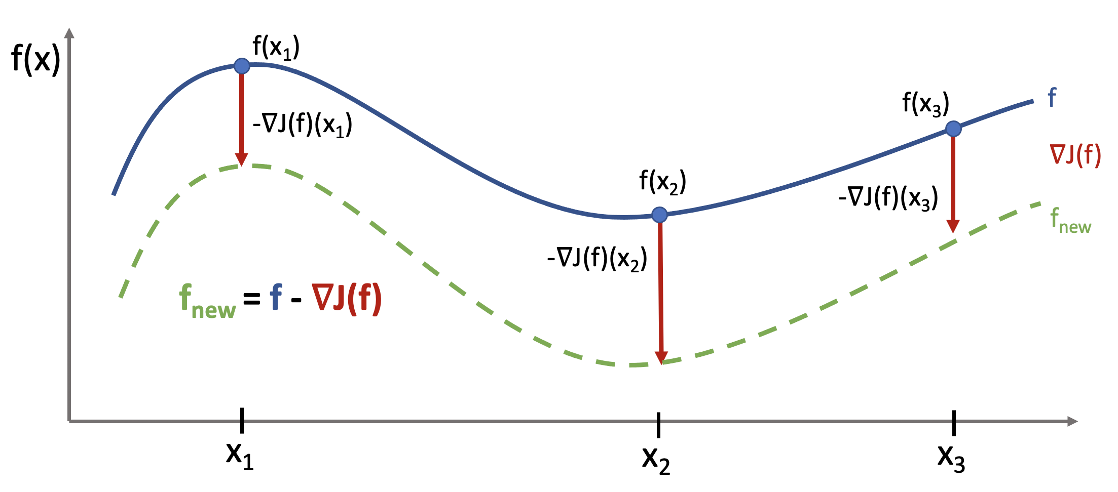
The functional gradient is a function that tells us how much we "move" $f(x)$ at each point $x$.
Given a good step size, the resulting new function will be closer to minimizing $J$.
Formally, the $x$-th entry of the vector $\nabla J (f)$ is the partial derivative $\frac{\partial J(f)}{\partial f(x)}$ of $J$ with respect to $f(x)$, the $x$-th component of $f$. $$ \frac{\partial J(f)}{\partial f(x)} = \frac{\partial}{\partial f(x)} \left( \mathbb{E}_{( x, y)\sim \mathbb{P}} \left[ L\left( y, f( x \right)) \right] \right) = \frac{\partial L(y, f)}{\partial f} \bigg\rvert_{f=f(x)} $$
So the functional gradient is $$ \nabla J (f) = \begin{bmatrix} \vdots \\ \frac{\partial L(y, f)}{\partial f} \bigg\rvert_{f=f(x)} \\ \vdots \\ \end{bmatrix}.$$ This is an infinite-dimensional vector indexed by $x$.
Supervised Learning Over Functions: Functional Gradient Descent
Previously, we optimized $J(\theta)$ using gradient descent via the update rule: $$\theta_t \gets \theta_{t-1} - \alpha_t \nabla J(\theta_{t-1})$$
We can now optimize our objective using gradient descent in functional space via the same update: $$f_t \gets f_{t-1} - \alpha_t \nabla J(f_{t-1}).$$
Supervised Learning Over Functions
After $T$ steps of $f_t \gets f_{t-1} - \alpha_t \nabla J(f_{t-1})$, we get a model of the form $$f_T = f_0-\sum_{t=0}^{T-1} \alpha_t \nabla J(f_{t})$$
- Recall that each $\nabla J(f_{t})$ is a function of $x$
- Therefore $f_T$ is a function of $x$ as well
- Because it's the result of gradient descent, $f_T$ will minimize $J$.
But recall that previously we were not able to compute $\nabla J(\theta) = \mathbb{E}_{( x, y)\sim \mathbb{P}} \left[ \nabla L\left( y, f_\theta( x) \right) \right]$ on infinite data and instead we used: $$ \hat \nabla J (\theta) = \frac{1}{m} \sum_{i=1}^m \nabla L\left( y^{(i)}, f_\theta( x^{(i)}) \right). $$
In our case, we also need to find an approximation $\hat \nabla J(f)$ to the functional gradient: $$ \nabla J(f) (x) = \frac{\partial J(f)}{\partial f(x)} = \frac{\partial L(y, f)}{\partial f} \bigg\rvert_{f=f(x)} $$
This is more challenging that before:
- $\nabla J(f) (x) = \frac{\partial L(y, f)}{\partial f} \bigg\rvert_{f=f(x)}$ is not an expectation so we can't approximate it with an average in the data.
- $\nabla J (f)$ is a function that we need to "learn" from $\mathcal{D}$. We will use supervised learning for this!
- We cannot represent $\nabla J(f)$ because it's a general function
- We cannot measure $\nabla J(f)$ at each $x$ (only at $n$ training points).
- Even if we could, the problem would be too unconstrained
Modeling Functional Gradients
We will address the above problem by learning a model of gradients.
- In supervised learning, we only have access to $n$ data points that describe the true $\mathcal{X} \to \mathcal{Y}$ mapping (call it $f^*$).
- We learn a model $f_\theta:\mathcal{X} \to \mathcal{Y}$ within $\mathcal{M}$ to approximate $f^*$.
- The model extrapolates beyond the training set. Given enough datapoints, $f_\theta$ learns a true mapping.
We will apply h same idea to gradients.
- We assume a model $g_{\theta_t} : \mathcal{X} \to R$ of the functional gradient $\nabla J(f_t)$ within a class $\mathcal{M}$. \begin{align*} g_{\theta_t} \in \mathcal{M} & & g_{\theta_t} \approx \nabla J(f_t) \end{align*}
- The model extrapolates beyond the training set. Given enough datapoints, $g_{\theta_t}$ learns $\nabla J(f_t)$.
Functional descent will then have the form: $$\underbrace{f_t(x)}_\text{new function} \gets \underbrace{f_{t-1}(x) - \alpha g_{\theta_{t-1}}(x)}_\text{old function - gradient step}.$$ If $g$ generalizes, this approximates $f_t \gets f_{t-1} - \alpha \nabla J(f_{t-1}).$
Fitting Functional Gradients
What does it mean to approximate a functional gradient $g \approx \nabla J(f)$ in practice? We can use standard supervised learning.
Suppose we have a fixed function $f$ and we want to estimate the functional gradient of $L$ $$\frac{\partial L(\text{y}, \text{f})}{\partial \text{f}} \bigg\rvert_{\text{f} = f(x)}.$$ at any $x \in \mathcal{X}$
- We define a loss $L_g$ (e.g., L2 loss) measure how well $g \approx \nabla J(f)$.
- We compute $\nabla J(f)$ on the training dataset: $$\mathcal{D}_g = \left\{ \left(x^{(i)}, \underbrace{\frac{\partial L(y^{(i)}, \text{f})}{\partial \text{f}} \bigg\rvert_{\text{f} = f(x^{(i)})}}_\text{functional derivative $\nabla_\textbf{f} J(\textbf{f})_i$ at $f(x^{(i)})$} \right), i=1,2,\ldots,n \right\} $$
- We train a model $g : \mathcal{X} \to \mathbb{R}$ on $\mathcal{D}_g$ to predict functional gradients at any $x$: $$ g(x) \approx \frac{\partial L(\text{y}, \text{f})}{\partial \text{f}} \bigg\rvert_{\text{f} = f_0(x)}.$$
Gradient Boosting
Gradient boosting is a procedure that performs functional gradient descent with approximate gradients.
Start with $f(x) = 0$. Then, at each step $t>1$:
- Create a training dataset $\mathcal{D}_g$ and fit $g_t(x^{(i)})$ using loss $L_g$: $$ g_t(x) \approx \frac{\partial L(\text{y}, \text{f})}{\partial \text{f}} \bigg\rvert_{\text{f} = f_0(x)}.$$
- Take a step of grad descent using approximate grads with step $\alpha_t$: $$f_t(x) = f_{t-1}(x) - \alpha_t \cdot g_t(x).$$
Interpreting Gradient Boosting
Notice how after $T$ steps we get an additive model of the form $$ f(x) = \sum_{t=1}^T \alpha_t g_t(x). $$ This looks like the output of a boosting algorithm!
- This works for any differentiable loss $L$.
- It does not require any mathematical derivations for new $L$.
Boosting vs. Gradient Boosting
Consider, for example, L2Boost, which optimizes the L2 loss $$ L(y, f) = \frac{1}{2}(y-f)^2. $$
At step $t$ we minimize $$\sum_{i=1}^n (r^{(i)}_t - g(x^{(i)}; \phi))^2, $$ where $r^{(i)}_t = y^{(i)} - f_{t-1}(x^{(i)})$ is the residual from the model at time $t-1$.
Observe that the residual $$r^{(i)}_t = y^{(i)} - f(x^{(i)})_{t-1}$$ is also the gradient of the $L2$ loss with respect to $f$ as $f(x^{(i)})$ $$r^{(i)}_t = \frac{\partial L(y^{(i)}, \text{f})}{\partial \text{f}} \bigg\rvert_{\text{f} = f_0(x)}$$
Many boosting methods are special cases of gradient boosting in this way.
Losses for Additive Models
We have seen several losses that can be used with the forward stagewise additive approach.
- The exponential loss $L(y,f) = \exp(-yf)$ gives us Adaboost.
- The log-loss $L(y,f) = \log(1+\exp(-2yf))$ is more robust to outliers.
- The squared loss $L(y,f) = (y-f)^2$ can be used for regression.
Losses for Gradient Boosting
Gradient boosting can optimize a wide range of losses.
- Regression losses:
- L2, L1, and Huber (L1/L2 interpolation) losses.
- Quantile loss: estimates quantiles of distribution of $p(y|x)$.
- Classification losses:
- Log-loss, softmax loss, exponential loss, negative binomial likelihood, etc.
Practical Considerations
When using gradient boosting these additional facts are useful:
- We most often use small decision trees as the learner $g_t$. Thus, input pre-processing is minimal.
- We can regularize by controlling tree size, step size $\alpha$, and using early stopping.
- We can scale-up gradient boosting to big data by subsampling data at each iteration (a form of stochastic gradient descent).
Algorithm: Gradient Boosting
- Type: Supervised learning (classification and regression).
- Model family: Ensembles of weak learners (often decision trees).
- Objective function: Any differentiable loss function.
- Optimizer: Gradient descent in functional space. Weak learner uses its own optimizer.
- Probabilistic interpretation: None in general; certain losses may have one.
Gradient Boosting: An Example
Let's now try running Gradient Boosted Decision Trees on a small regression dataset.
First we create the dataset.
# https://scikit-learn.org/stable/auto_examples/ensemble/plot_gradient_boosting_quantile.html
X = np.atleast_2d(np.random.uniform(0, 10.0, size=100)).T
X = X.astype(np.float32)

# Create dataset
f = lambda x: x * np.sin(x)
y = f(X).ravel()
dy = 1.5 + 1.0 * np.random.random(y.shape)
noise = np.random.normal(0, dy)
y += noise

# Visualize it
xx = np.atleast_2d(np.linspace(0, 10, 1000)).T
plt.plot(xx, f(xx), 'g:', label=r'$f(x) = x\,\sin(x)$')
plt.plot(X, y, 'b.', markersize=10, label=u'Observations')
[<matplotlib.lines.Line2D at 0x12ed61898>]

Next, we train a GBDT regressor.
from sklearn.ensemble import GradientBoostingRegressor

alpha = 0.95
clf = GradientBoostingRegressor(loss='ls', alpha=alpha,
                                n_estimators=250, max_depth=3,
                                learning_rate=.1, min_samples_leaf=9,
                                min_samples_split=9)
clf.fit(X, y)
GradientBoostingRegressor(alpha=0.95, min_samples_leaf=9, min_samples_split=9,
                          n_estimators=250)
We may now visualize its predictions
y_pred = clf.predict(xx)
plt.plot(xx, f(xx), 'g:', label=r'$f(x) = x\,\sin(x)$')
plt.plot(X, y, 'b.', markersize=10, label=u'Observations')
plt.plot(xx, y_pred, 'r-', label=u'Prediction')
[<matplotlib.lines.Line2D at 0x12c98e438>]

Pros and Cons of Gradient Boosting
Gradient boosted decision trees (GBTs) are one of the best off-the-shelf ML algorithms that exist, often on par with deep learning.
- Attain state-of-the-art performance. GBTs have won the most Kaggle competitions.
- Require little data pre-processing and tuning.
- Work with any objective, including probabilistic ones.
Their main limitations are:
- GBTs don't work with unstructured data like images, audio.
- Implementations not as flexible as modern neural net libraries.