Congratulations on Finishing Applied Machine Learning!
This is our last machine learning lecture, in which we will do an overview of the diffrent algorithms seen in the course.
Announcements
- There is no lecture this Thursday
- I am holding extra office hours for the project next week
- Stay tuned for details
- Project is due on December 12
- Please write your course reviews!
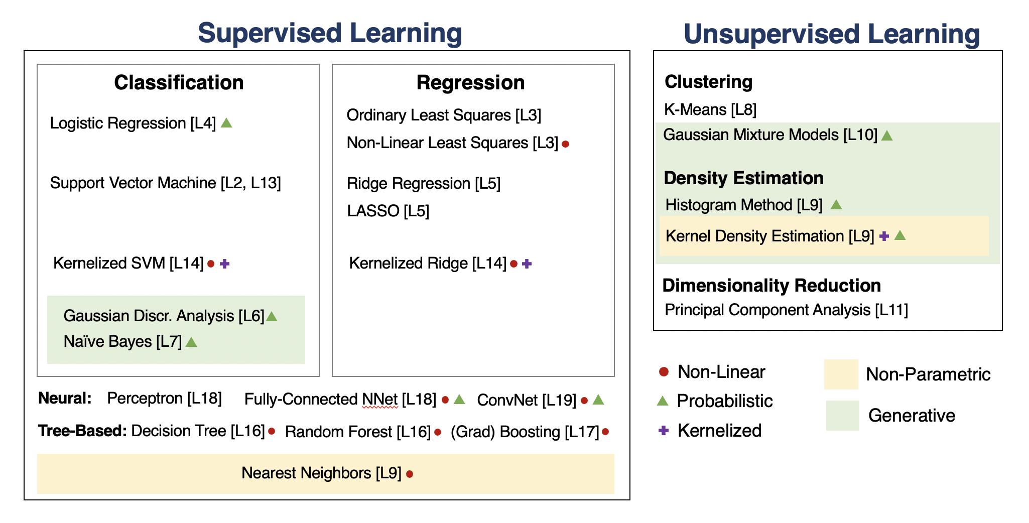
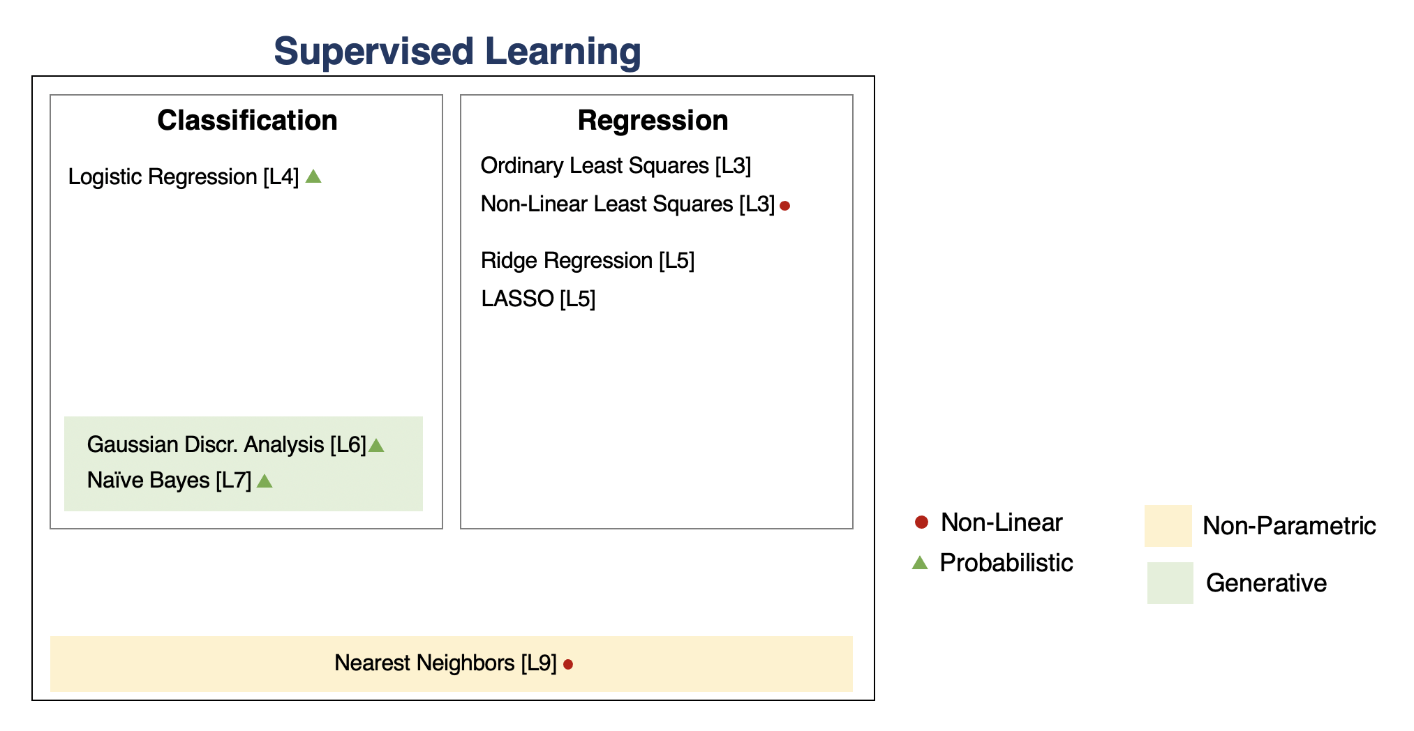
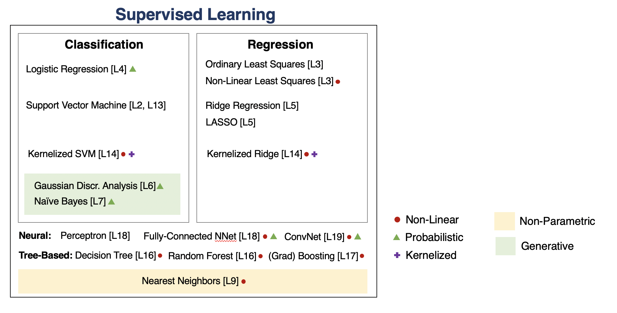
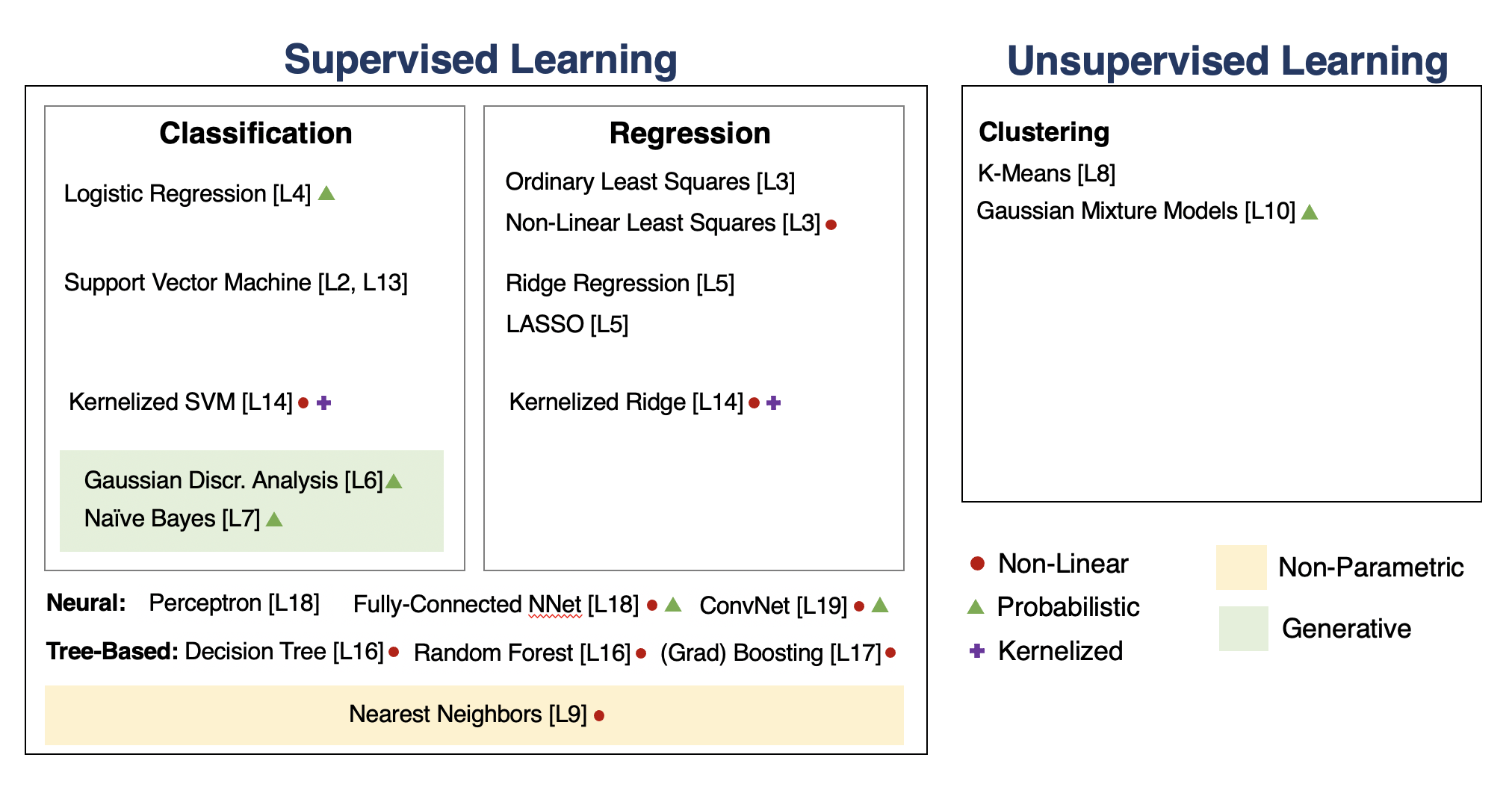
A Map of Applied Machine Learning
We will go through the following map of algorithms from the course.
Key Idea: Components of Supervised Learning
To apply supervised learning, we define a dataset and a learning algorithm.
$$ \underbrace{\text{Dataset}}_\text{Features, Attributes, Targets} + \underbrace{\text{Learning Algorithm}}_\text{Model Class + Objective + Optimizer } \to \text{Predictive Model} $$
The output is a predictive model that maps inputs to targets. For instance, it can predict targets on new inputs.
Example: Linear Regression
In linear regression, we fit a model $$ f_\theta(x) := \theta^\top \phi(x) $$ that is linear in $\theta$.
The features $\phi(x) : \mathbb{R} \to \mathbb{R}^p$ are non-linear may non-linear in $x$ (e.g., polynomial features), allowing us to fit complex functions.
We define the least squares objective for the model as: $$ J(\theta) = \frac{1}{2} \sum_{i=1}^n (y^{(i)} - \theta^\top x^{(i)})^2 = \frac{1}{2} (X \theta - y)^\top (X \theta - y) $$
We can set the gradient to zero to obtain the normal equations: $$ (X^\top X ) \theta = X^\top y. $$
Hence, the value $\theta^*$ that minimizes this objective is given by: $$ \theta^* = (X^\top X)^{-1} X^\top y.$$
Key Ideas: Overfitting & Underfitting
Overfitting is one of the most common failure modes of machine learning.
- A very expressive model (a high degree polynomial) fits the training dataset perfectly.
- The model also makes wildly incorrect prediction outside this dataset, and doesn't generalize.
We can measure overfitting and underfitting by estimating accuracy on held out data and comparing it to the training data.
- If training perforance is high but holdout performance is low, we are overfitting.
- If training perforance is low and holdout performance is low, we are underfitting.
We will see many ways of dealing with overftting, but here are some ideas:
- Use a simpler model family (linear models vs. neural nets)
- Keep the same model, but collect more training data
- Modify the training process to penalize overly complex models.
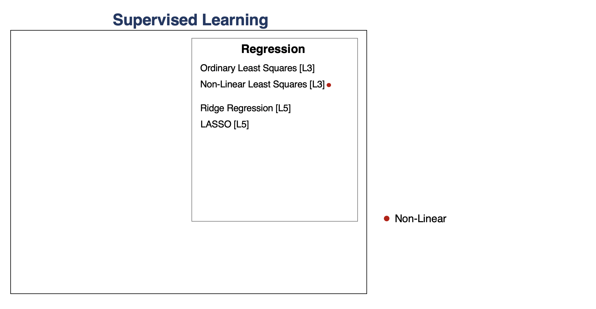
Key Idea: Regularization
The idea of regularization is to penalize complex models that may overfit the data.
Regularized least squares optimizes the following objective (Ridge). $$ J(\theta) = \frac{1}{2n} \sum_{i=1}^n \left( y^{(i)} - \theta^\top x^{(i)} \right)^2 + \frac{\lambda}{2} \cdot ||\theta||_2^2. $$ If we use the L1 norm, we have the LASSO.
To find optimal Ridge parameters, we can set the gradient to zero to obtain the normal equations: $$ (X^\top X + \lambda I) \theta = X^\top y. $$
Hence, the value $\theta^*$ that minimizes this objective is given by: $$ \theta^* = (X^\top X + \lambda I)^{-1} X^\top y.$$
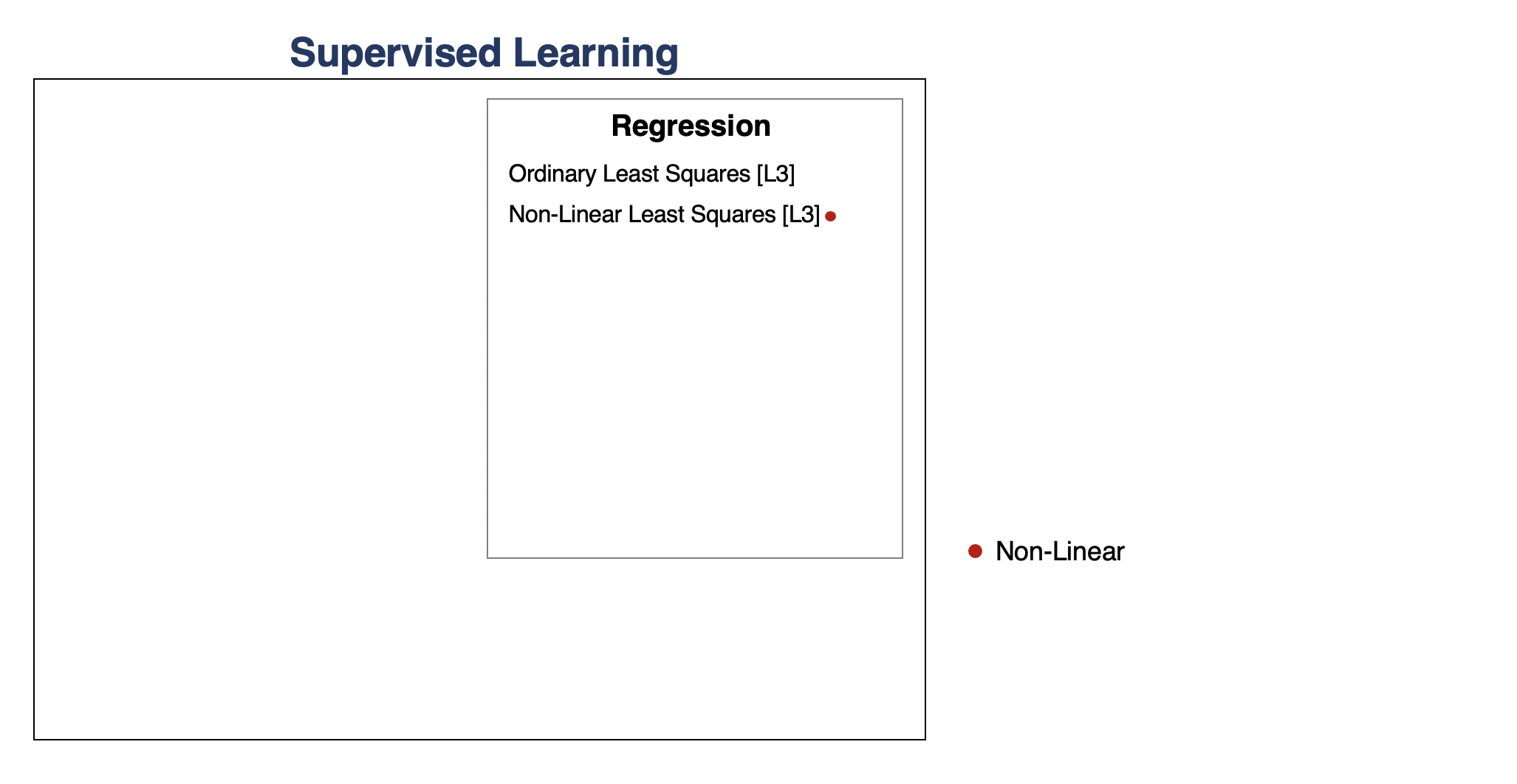
Regression vs. Classification
Consider a training dataset $\mathcal{D} = \{(x^{(1)}, y^{(1)}), (x^{(2)}, y^{(2)}), \ldots, (x^{(n)}, y^{(n)})\}$.
We distinguish between two types of supervised learning problems depnding on the targets $y^{(i)}$.
- Regression: The target variable $y \in \mathcal{Y}$ is continuous: $\mathcal{Y} \subseteq \mathbb{R}$.
- Classification: The target variable $y$ is discrete and takes on one of $K$ possible values: $\mathcal{Y} = \{y_1, y_2, \ldots y_K\}$. Each discrete value corresponds to a class that we want to predict.
Example: Logistic Regression
Logistic regression fits models of the form: $$ f(x) = \sigma(\theta^\top x) = \frac{1}{1 + \exp(-\theta^\top x)}, $$ where $$ \sigma(z) = \frac{1}{1 + \exp(-z)} $$ is known as the sigmoid or logistic function.
Example: K-Nearest Neighbors
At inference time, we receive a query point $x'$ and we want to predict its label $y'$.
- Given a query datapoint $x'$, find the $K$ training examples $\mathcal{N} = \{(x^{(1)}, y^{(1)}), (x^{(2)}, y^{(2)}), \ldots, (x^{(K)}, y^{(K)})\}$ that are closest to $x'$.
- Return $y_\mathcal{N}$, the consensus label of the neighborhood $\mathcal{N}$.
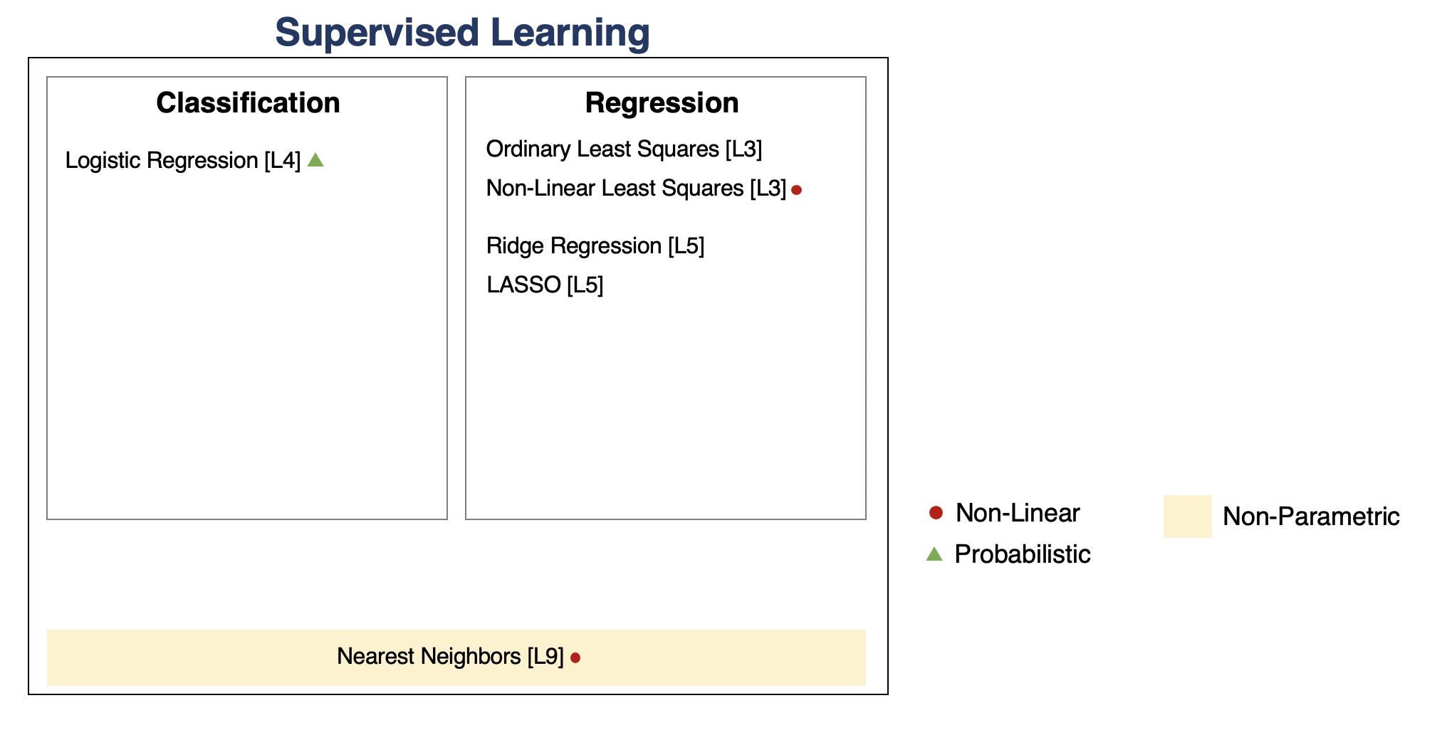
Key Idea: Parametric vs. Non-Parametric Models
Nearest neighbors is an example of a non-parametric model.
- A parametric model $f_\theta(x) : \mathcal{X} \times \Theta \to \mathcal{Y}$ is defined by a finite set of parameters $\theta \in \Theta$ whose dimensionality is constant with respect to the dataset
- In a non-parametric model, the function $f$ uses the entire training dataset to make predictions, and the complexity of the model increases with dataset size.
- Non-parametric models have the advantage of not loosing any information at training time.
- However, they are also computationally less tractable and may easily overfit the training set.
Probabilistic Models
Many supervised learning models have a probabilistic interpretation. Often a model $f_\theta$ defines a probability distribution of the form
$$ P_\theta(y|x) : \underbrace{\mathcal{X}}_\text{input} \to \underbrace{(\mathcal{Y} \to [0,1])}_\text{probability P(y|x) over $\mathcal{Y}$} $$
We refer to these as probabilistic models.
For example, our logistic model defines ("parameterizes") a probability distribution $P_\theta(y|x) : \mathcal{X} \to ( \mathcal{Y} \to [0,1])$ as follows:
\begin{align*} P_\theta(y=1 | x) & = \sigma(\theta^\top x) \\ P_\theta(y=0 | x) & = 1-\sigma(\theta^\top x). \end{align*}
Key Idea: Discriminative vs. Generative Models
There are two types of probabilistic models: generative and discriminative. \begin{align*} \underbrace{P_\theta(x,y) : \mathcal{X} \times \mathcal{Y} \to [0,1]}_\text{generative model} & \;\; & \underbrace{P_\theta(y|x) : \mathcal{X} \to ( \mathcal{Y} \to [0,1])}_\text{discriminative model} \end{align*}
We can obtain predictions from generative models via $\max_y P_\theta(x,y)$.
- A generative approach first builds a model of $x$ for each class: $$ P_\theta(x | y=k) \; \text{for each class $k$}.$$ $P_\theta(x | y=k)$ scores $x$ according to how well it matches class $k$.
- A class probability $P_\theta(y=k)$ encoding our prior beliefs $$ P_\theta(y=k) \; \text{for each class $k$}.$$ These are often just the % of each class in the data.
We choose the class whose model fits $x$ best.
Example: Gaussian Discriminant Analysis
Gaussian Discriminant Analysis defines a model $P_\theta$ as follows:
- The conditional probability $P(x\mid y=k)$ of the data under class $k$ is a multivariate Gaussian $\mathcal{N}(x; \mu_k, \Sigma_k)$ with mean and covariance $\mu_k, \Sigma_k$.
- The distribution over classes is Categorical, denoted $\text{Categorical}(\phi_1, \phi_2, ..., \phi_K)$. Thus, $P_\theta(y=k) = \phi_k$.
Example: Bernoulli Naive Bayes
Bernoulli Naive Bayes defines a model $P_\theta$ as follows:
- The conditional probability $P(x\mid y=k)$ of the data under class $k$ is $$P_\theta(x|y=k) = \prod_{j=1}^d P(x_j \mid y=k),$$ where each $P_\theta(x_j \mid y=k)$ is a $\text{Bernoullli}(\psi_{jk})$. This is good for bag of words data.
- The distribution over classes is Categorical, denoted $\text{Categorical}(\phi_1, \phi_2, ..., \phi_K)$. Thus, $P_\theta(y=k) = \phi_k$.
Key Idea: Maximum Likelihood Learning
We can learn a generative model $P_\theta(x, y)$ by maximizing the maximum likelihood:
$$ \max_\theta \frac{1}{n}\sum_{i=1}^n \log P_\theta({x}^{(i)}, y^{(i)}). $$
This seeks to find parameters $\theta$ such that the model assigns high probability to the training data.
Key Idea: The Max-Margin Principle
Logistic regression and Naive Bayes are both linear classifiers. However, they yield different decision boundaries.
Intuitively, we want to select linear decision boundaries with high margin: every point is as far as possible from the decision boundary.
import numpy as np
import pandas as pd
from sklearn import datasets

# Load the Iris dataset
iris = datasets.load_iris(as_frame=True)
iris_X, iris_y = iris.data, iris.target

# subsample to a third of the data points
iris_X = iris_X.loc[::4]
iris_y = iris_y.loc[::4]

# create a binary classification dataset with labels +/- 1
iris_y2 = iris_y.copy()
iris_y2[iris_y2==2] = 1
iris_y2[iris_y2==0] = -1

# print part of the dataset
pd.concat([iris_X, iris_y2], axis=1).head()
| sepal length (cm) | sepal width (cm) | petal length (cm) | petal width (cm) | target | |
|---|---|---|---|---|---|
| 0 | 5.1 | 3.5 | 1.4 | 0.2 | -1 |
| 4 | 5.0 | 3.6 | 1.4 | 0.2 | -1 |
| 8 | 4.4 | 2.9 | 1.4 | 0.2 | -1 |
| 12 | 4.8 | 3.0 | 1.4 | 0.1 | -1 |
| 16 | 5.4 | 3.9 | 1.3 | 0.4 | -1 |
# https://scikit-learn.org/stable/auto_examples/neighbors/plot_classification.html
%matplotlib inline
import matplotlib.pyplot as plt
plt.rcParams['figure.figsize'] = [12, 4]
import warnings
warnings.filterwarnings("ignore")

# create 2d version of dataset and subsample it
X = iris_X.to_numpy()[:,:2]
x_min, x_max = X[:, 0].min() - .5, X[:, 0].max() + .5
y_min, y_max = X[:, 1].min() - .5, X[:, 1].max() + .5
xx, yy = np.meshgrid(np.arange(x_min, x_max, .02), np.arange(y_min, y_max, .02))

# Plot also the training points
p1 = plt.scatter(X[:, 0], X[:, 1], c=iris_y2, s=60, cmap=plt.cm.Paired)
plt.xlabel('Petal Length')
plt.ylabel('Petal Width')
plt.legend(handles=p1.legend_elements()[0], labels=['Setosa', 'Not Setosa'], loc='lower right')
<matplotlib.legend.Legend at 0x12b41fb00>

from sklearn.linear_model import Perceptron, RidgeClassifier
from sklearn.svm import SVC
models = [SVC(kernel='linear', C=10000), Perceptron(), RidgeClassifier()]

def fit_and_create_boundary(model):
    model.fit(X, iris_y2)
    Z = model.predict(np.c_[xx.ravel(), yy.ravel()])
    Z = Z.reshape(xx.shape)
    return Z

plt.figure(figsize=(12,3))
for i, model in enumerate(models):
    plt.subplot('13%d' % (i+1))
    Z = fit_and_create_boundary(model)
    plt.pcolormesh(xx, yy, Z, cmap=plt.cm.Paired)

    # Plot also the training points
    plt.scatter(X[:, 0], X[:, 1], c=iris_y2, edgecolors='k', cmap=plt.cm.Paired)
    if i == 0:
        plt.title('Good Margin')
    else:
        plt.title('Bad Margin')
    plt.xlabel('Sepal length')
    plt.ylabel('Sepal width')

plt.show()

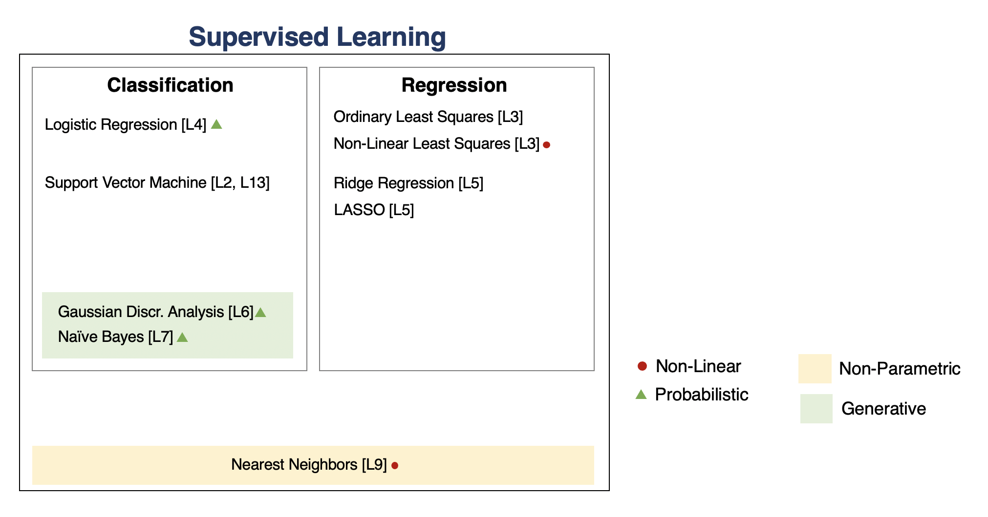
Example: Support Vector Machines
Support Vector Machines fit linear models of the form
\begin{align*} f_\theta(x) = \theta^\top \phi(x) + \theta_0 \end{align*}
such as to find the maximum margin hyperplane.
SVM: Constrained Primal
Recall that the the max-margin hyperplane can be formualted as the solution to the following primal optimization problem. \begin{align*} \min_{\theta,\theta_0, \xi}\; & \frac{1}{2}||\theta||^2 + C \sum_{i=1}^n \xi_i \; \\ \text{subject to } \; & y^{(i)}((x^{(i)})^\top\theta+\theta_0)\geq 1 - \xi_i \; \text{for all $i$} \\ & \xi_i \geq 0 \end{align*}
SVM: Unconstrained Primal
We can turn our optimization problem into an unconstrained form: $$ \min_{\theta,\theta_0}\; \sum_{i=1}^n \underbrace{\left(1 - y^{(i)}\left((x^{(i)})^\top\theta+\theta_0\right)\right)^+}_\text{hinge loss} + \underbrace{\frac{\lambda}{2}||\theta||^2}_\text{regularizer} $$
- The hinge loss penalizes incorrect predictions.
- The L2 regularizer ensures the weights are small and well-behaved.
SVM: Dual
The solution to the primal problem also happens to be given by the following dual problem: \begin{align*} \max_{\lambda} & \sum_{i=1}^n \lambda_i - \frac{1}{2} \sum_{i=1}^n \sum_{k=1}^n \lambda_i \lambda_k y^{(i)} y^{(k)} (x^{(i)})^\top x^{(k)} \\ \text{subject to } \; & \sum_{i=1}^n \lambda_i y^{(i)} = 0 \\ & C \geq \lambda_i \geq 0 \; \text{for all $i$} \end{align*}
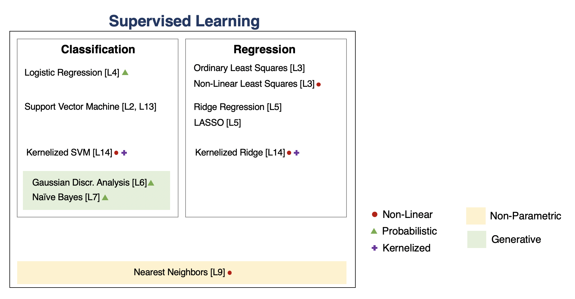
Key Idea: The Kernel Trick
Many algorithms in machine learning only involve dot products $\phi(x)^\top \phi(z)$ but not the features $\phi$ themselves.
We can often compute $\phi(x)^\top \phi(z)$ very efficiently for complex $\phi$ using a kernel function $K(x,z) = \phi(x)^\top \phi(z)$. This is the kernel trick.
Example: The Kernel Trick in SVMs
Notice that in the SVM dual, the features $\phi(x)$ are never used directly. Only their dot product is used.
\begin{align*} J(\lambda) &= \sum_{i=1}^n \lambda_i - \frac{1}{2} \sum_{i=1}^n \sum_{k=1}^n \lambda_i \lambda_k y^{(i)} y^{(k)} \phi(x^{(i)})^\top \phi(x^{(k)}) \end{align*}
If we can compute the dot product efficiently, we can potentially use very complex features.
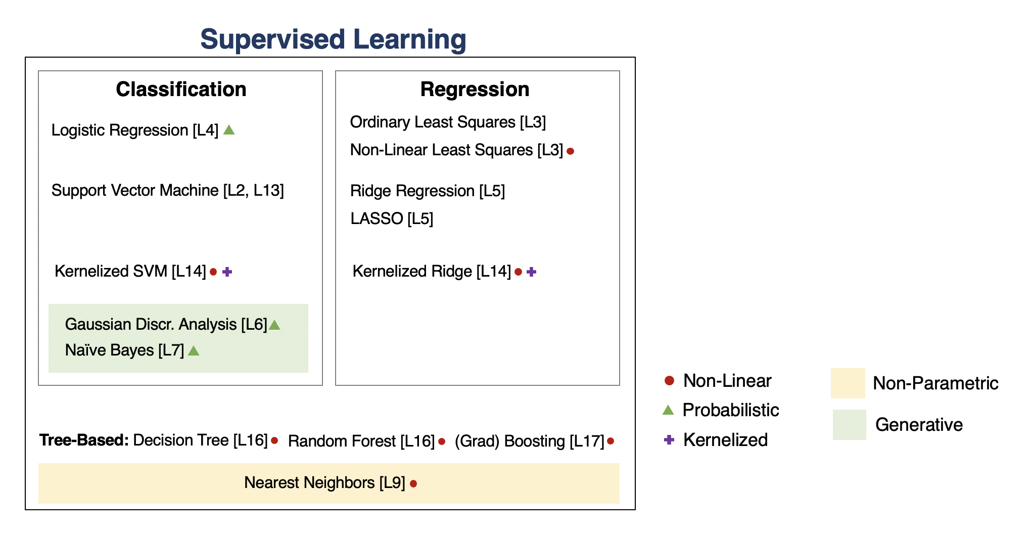
Tree-Based Models
Decision trees output target based on a tree of human-interpretable decision rules.
- Random forests combine large trees using bagging to reduce overfitting.
- Boosted trees combine small trees to reduce underfitting.
Neural Networks
Neural network models are inspired by the brain.
- A Perceptron is an artificial model of a neuron.
- MLP stack multiple layers of artifical neurons.
- ConvNets tie the weights of neighboring neurons into receptive fields that implement the convolution operation.
Unsupervised Learning
We have a dataset without labels. Our goal is to learn something interesting about the structure of the data:
- Clusters hidden in the dataset.
- A low-dimensional representation of the data.
- Recover the probability density that generated the data.
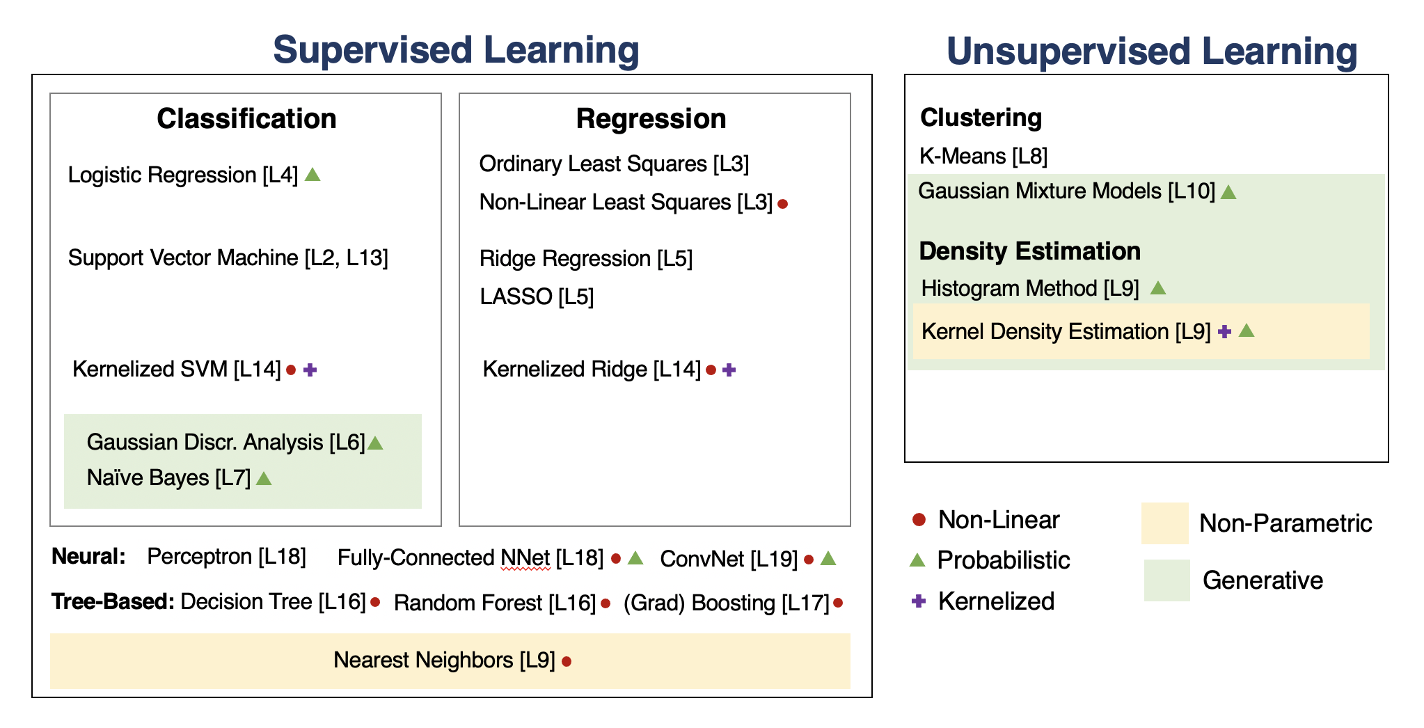
Key Idea: Density Estimation
The problem of density estimation is to approximate the data distribution $P_\text{data}$ with the model $P$. $$ P \approx P_\text{data}. $$
It's also a general learning task. We can solve many downstream tasks using a good model $P$:
- Outlier and novelty detection
- Generating new samples $x$
- Visualizing and understanding the structure of $P_\text{data}$
In Kernel density estimation we will fit a model of the form $$P(x) \propto \sum_{i=1}^n K(x, x^{(i)})$$ One example is the Gaussian kernel $K(x,z; \delta) \propto \exp(-||x-z||^2/2\delta^2)$.
Key Idea: Clustering & Gaussian Mixtures
We can perform clustering via density estimation with a GMM model. $$P_\theta (x,z) = P_\theta (x | z) P_\theta (z)$$
- $z \in \mathcal{Z} = \{1,2,\ldots,K\}$ is discrete and follows a categorical distribution $P_\theta(z=k) = \phi_k$.
- $x \in \mathbb{R}$ is continuous; conditioned on $z=k$, it follows a Normal distribution $P_\theta(x | z=k) = \mathcal{N}(\mu_k, \Sigma_k)$.
The parameters $\theta$ are the $\mu_k, \Sigma_k, \phi_k$ for all $k=1,2,\ldots,K$.
Intuitively, a GMM represents well the two clusters in the geyser dataset:
| Raw data | Single Gaussian | Mixture of Gaussians |
|---|---|---|
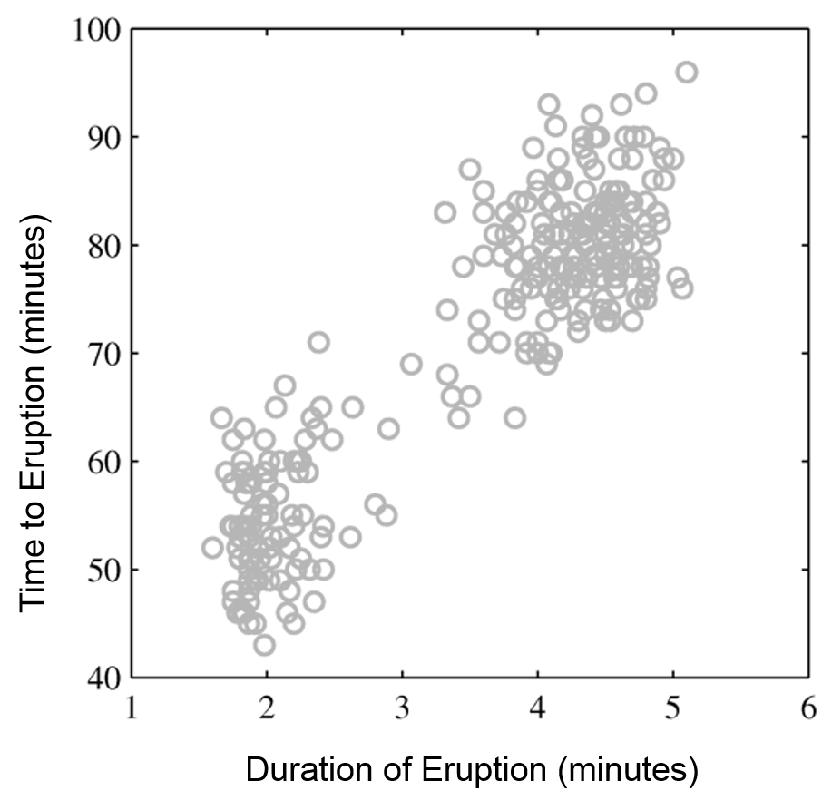 |
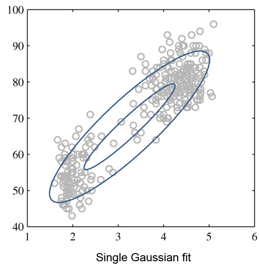 |
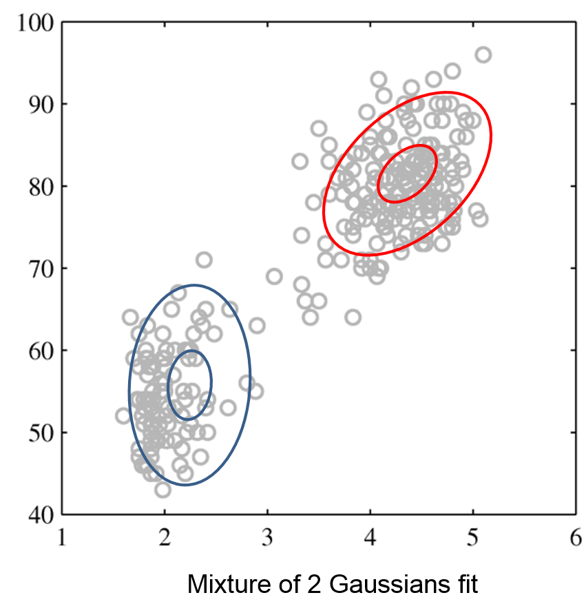 |
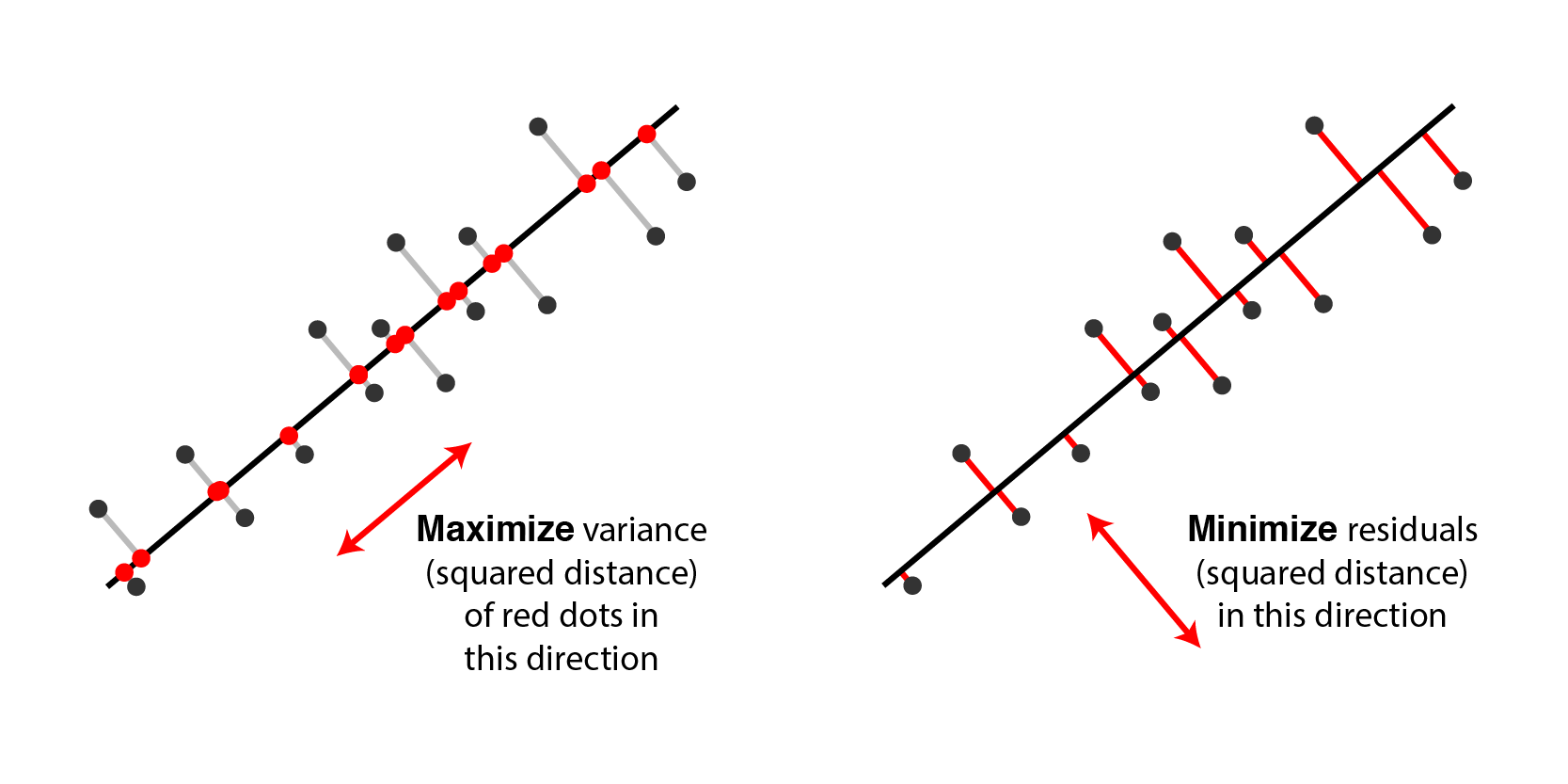
Key Idea: Linear Dimensionality Reduction
Suppose $\mathcal{X} = \mathbb{R}^d$ and $\mathcal{Z} = \mathbb{R}^p$ for some $p < d$. The transformation $$f_\theta : \mathcal{X} \to \mathcal{Z}$$ is a linear function with parameters $\theta = W \in \mathbb{R}^{d \times p}$: $$ z = f_\theta(x) = W^\top \cdot x. $$ The latent dimension $z$ is obtained from $x$ via a matrix $W$.
We find $W$ using one of the following equivalent objectives (figure credit: Alex Williams)

How To Decide Which Algorithm to Use
One factor is how much data you have. In the small data (<10,000) regime, consider:
- Linear models with hand-crafted features (LASSO, LR, NB, SVMs)
- Kernel methods often work best (e.g., SVM + RBF kernel)
- Non-parametric methods (kernels, nearest neighbors) are also powerful
In the big data regime,
- If using "high-level" features, gradient boosted trees are state-of-the-art
- When using "low-level" representations (images, sound signals), neural networks work best
- Linear models with good features are also good and reliable
Some additional advice:
- If interpretability matters, use decision trees or LASSO.
- When uncertainty estimates are important use probabilistic methods.
- If you know the data generating process, use generative models.
What's Next? Ideas for Courses
Consider the following courses to keep learning about ML:
- Graduate courses in the Spring semester at Cornell (generative models, NLP, etc.)
- Masters courses: Deep Learning, ML Engineering, Data Science, etc.
- Online courses, e.g. Full Stack Deep Learning
What's Next? Ideas for Research
In order to get involved in research, I recommend:
- Contacting research groups at Cornell for openings
- Watching online ML tutorials, e.g. NeurIPS
- Reading and implementing ML papers on your own
What's Next? Ideas for Industry Projects
Finally, a few ideas for how to get more practice applying ML in the real world:
- Participate in Kaggle competitions and review solutions
- Build an open-source project that you like and host it on Github
Thank You For Taking Applied Machine Learning!
